IEEE Visualization 2008 Design Contest

This page describes the format and semantics of the data files for the contest. See the Data Download page to get copies of the actual data.

Data Set Description

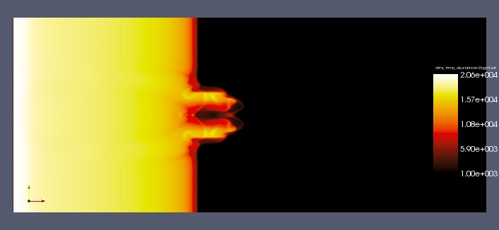
Numerical simulations of the first stars in the universe reveal that they formed in isolation several hundred million years before the first primitive galaxies were assembled and that they were very massive: 100 - 500 solar masses. With surface temperatures greater than 100,000 K they were millions of times brighter than the sun, with most of their light in the form of hard (energetic) UV radiation. These UV photons could not simply stream into the universe because they were capable of ionizing H and He into ions and free electrons. Instead, they advanced behind an abrupt wall of radiation known as an ionization front (or I-front) at well below the speed of light. The I-front itself is the extremely thin layer separating the hot (20,000 K), completely ionized gas from the cold (72 K), neutral gas beyond the front.

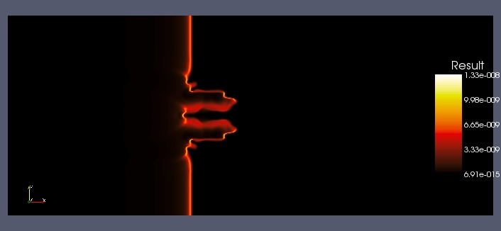
The radiation wave at first propagates supersonically through space, leaving gas undisturbed in its wake, but then slows as it recedes from the star. The hot ionized gas drives a shock that overtakes and pushes past the front, and the radiation wave is subsonic thereafter. The shock driven by the radiation front snowplows ambient gas into a dense layer that can erupt in violent dynamical instabilities as shown in the figure below from [1]. There, the initially planar I-front sweeps over a spherical blob of gas and is deformed by it. The dimple destabilizes and fragments into a jet, a phenomenon known as a shadow instability. I-front instabilities endow nebulae in the galaxy today with spectacular morphologies (such as the "pillars of creation' in the Eagle Nebula) and recent numerical work confirms they were also present in those of the first stars.

Besides being aesthetically pleasing, instabilities in primordial radiation fronts clumped gas that might have later collapsed gravitationally into the next generation of stars, accelerating the formation of the first galaxies. While we have numerical proof of their existence, much remains unknown about these beautiful structures in the primeval universe and how they may have fostered subsequent star formation. The scientists need your help as visualization experts to unravel the role of I-front instabilities in structure formation in the early universe.

The scientists performed three-dimensional radiation hydrodynamical calculations of ionization front instabilities in which multifrequency radiative transfer is coupled to eight species primordial chemistry. They simulated ten scalar fields: particle density, temperature, and 8 chemical species. The velocity field is also simulated. Detailed information about the simulation and results found to date are in [1] and [2].

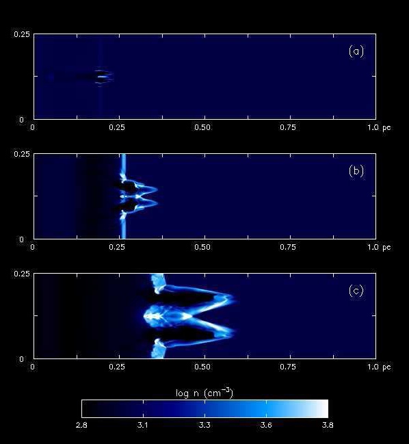
The figure above, from [1], shows a shadow instability. The images above show a 2D slice through the data set of the logarithm of density over time as the instability progresses towards the right. Figure (a) is from 1.9 thousand years (kyr) into the simulation, (b) is from 4.9 kyr, and (c) from 12.6 kyr.

The scientists have not yet seen a 3D animation of the density distribution over time, much less a multivariate visualization of the interactions between multiple data sets over time. This is your chance to be part of new discoveries about the way the universe formed!

Region

The simulation propagates through a volume of space that is 0.6 by 0.25 by 0.25 parsecs on a side. Element (0,0,0) is at the lower bottom corner of the volume; it is a right-handed coordinate system with X being the longest axis and Y and Z being the same size. There are 200 simulation time steps covering 25.37 thousand years.

Data Format

Coordinate System

In this simulation, the region is treated as a flat Cartesian box. This volume is divided into regular squares with a 0.001 parsec spacing in all directions in the pre-decimated mesh, creating a 600x248x248 point regular mesh. This results in a mesh consisting of 36.9 million regular cubes. The output data is saved as single file per time step.

Time: The original simulation stored the state of the entire volume approximately every 126.8 years. This was calculated for a total of 25,370 years for a total of 200 time steps. The actual time corresponding to each time index is stored here; the values range from around 126 years to around 128 years between steps.

Data Layout

All simulation data is saved in ASCII format. The data is saved in files with no headers. To enable proper interpretation of the data, we specify the x,y,z dimensions of the mesh and data types that the floating points represent, the units of the data, and the order in which the indices change.

There are two types of data here: scalar (temperature, mass density, chemical species), and vector (velocity). All of the scalar fields for one time step are stored in a single gzip-compressed ASCII file named multifield.XXXX.txt.gz, where XXXX is the time step index (starting at 0000).

Line format: The values for each grid cell are laid out in a line that ends with a single ASCII newline (character 10, 0a in hexadecimal) except the last line, which has no terminating character. Each line has ten values, separated by a single space. There is no space between the last character of the last value and the newline ending the line. Each value is represented in scientific notation an optional '-' sign, then one digit, then a decimal point, then three more digits, then 'E', then + or -, then a three-digit exponent. An example line (the first line from the first line from multifield.0030.txt) is shown here:

8.563E+002 2.051E+004 4.180E-004 7.596E-001 5.260E-005 6.898E-002 1.710E-001 8.053E-011 2.686E-013 8.650E-012

There is one such line for every grid point in each file. There is one file per time step in the simulation. The X indices value most rapidly, then Y, then Z; the first line in the file refers to element (0,0,0); the second to element (1,0,0); the last to element (599,247,247).

The order of the ten columns on each line is:

  1. total particle density (# of particles/cm^3)
  2. gas temperature (degrees Kelvin)
  3. H mass abundance
  4. H+ mass abundance
  5. He mass abundance
  6. He+ mass abundance
  7. He++ mass abundance
  8. H- mass abundance
  9. H_2 mass abundance
  10. H_2+ mass abundance

Density Data Set

This is the total number of particles (of any type) per cubic centimeter. This and all scalar fields are sampled at the cell center.

Gas Temperature

Temperature is stored in degrees Kelvin. Ambient gas is very cool (72 K). Shocked gas is around 2000-3000 K. Ionized gas is much hotter: 20,000 Kelvin). Temperature thus indicates where shock waves and radiation are present. This and all scalar fields are sampled at the cell center.

Chemical Species Data Sets

The chemical-species data values are relative abundancies of the eight different chemical species being simulated (H, H+, He, He+, He++, H-, H_2, and H_2+). These values are normalized per grid cell so that they sum to 1. This is the fraction of total mass composed of each of these elements. This and all scalar fields are sampled at the cell center.

Velocity Data Set

The velocity data set is stored in a separate gzip-compressed file per time step, named velocity.XXXX.txt.gz, where XXXX is the time-step index (starting at 0000).

There are three components of velocity, X, Y, and Z in km/s. They are stored sequentially in the line. The are also separated and denoted as the values in the scalar-field file. Although the scalar data is cell-centered, the velocity data has each component centered on its respective lower face of the cell (x-velocities are centered on the lower x face, y-velocities on the lower y face, and z-velocities on the lower z face). An example line (from velocity.0030.txt) follows:

8.555E-012 -2.576E-040 9.431E-016

The velocity data set is not of direct relevance to the questions being asked by the scientists, but the magnitude of the curl of the velocity field can be used as an estimator of turbulence, which is of direct interest. The formula for the three components of the curl vector field is:

  • curl_x(i,j,k) = (vz(i,j+1,k) - vz(i,j,k) - vy(i,j,k+1) + vy(i,j,k)) / 0.001
  • curl_y(i,j,k) = (vx(i,j,k+1) - vx(i,j,k) - vz(i+1,j,k) + vz(i,j,k)) / 0.001
  • curl_z(i,j,k) = (vy(i+1,j,k) - vy(i,j,k) - vx(i,j+1,k) + vx(i,j,k)) / 0.001

Note that since velocities are face-centered in ZEUS-MP the derivative terms above (and therefore the components of the curl) are cell-centered. The vorticity (magnitude of the curl) is thus also cell centered.

Example Readers and Images

Scalar Data: A header to add to a multifield file that will convert it into a VTK structured grid file can be found here. (Note: the resulting data set is quite large and my laptop runs out of memory when trying to open the whole file. See the next paragraph for how to reduce the size by extracting a single field.)

C code to parse the input file and write out a VTK file with just the density values can be found here. The result of running this on the file from time index 30 (compressed into a ZIP file) can be found here. A faster-loading Paraview data format file of the same data written with Paraview 3.2.1 (www.paraview.org) can be found here. This data set can be loaded on my laptop; the Paraview binary data file loads much faster (and can be opened by the open-source Paraview application versions 2.4 and up).

The image below shows a view of the isosurface of the density data set above taken at the density level 2000 at timestep 30.

Vector Data: A header to add to a multifield file that will convert it into a VTK structured grid file can be found here. (Note: the resulting data set was too large to be loaded on my laptop; for an alernative path that uses a binary file, see the paragraph below.)

C code to parse a velocity file and produce a binary file that has three floats for each line in the original ASCII file can be found here. The resulting binary file (found here in a 157-MB zip file) can be read into Paraview by manually specifying the raw binary file reader and filling in: origin (0,0,0), spacing (0.001, 0.001, 0.001), extent (0:599, 0:247, 0:247), num components (3), float, and the appropriate endianness (little on a PC, big on a sun).

The image below shows the results from applying the glyph filter in Paraview 2.4 to the loaded binary file, using the default settings, at timestep 30.

Example Derived Data Sets

Curl Magnitude: A C program to read the velocity field and export both a VTK file and a binary file that records the curl magnitude (as defined above) can be found here. A compressed copy of the binary file can be found here.

The image below shows the results of applying an isosurface at value 3500 to the VTK curl magnitude file calculated using the curl-magnitude-calculation program on the velocity field for timestep 0030. (Note that prior to 7/14/2008, this image was incorrect because the example curl-calculation code was incorrect.)

Z Slice: To extract the Z=124 slice (one of the two nearest the center in Z) from a single compressed volumetric multifield file, use the following shell script in Unix or Cygwin (example is for time step 30):

  • gunzip < multifield.0030.txt.gz | tail +18451200 | head -148800 > multifield.0030.zslice.txt

To convert the resulting text file into a VTK-readible slice of 10-field data, prepend this file to it.

  • cat vtk_multifield_slice_header.txt multifield.0030.zslice.txt > multifield.0030.zslice.vtk

A zip file containing the resulting VTK file can be downloaded here.

The image below shows the 0th (density) field from a Z slice taken at slice 124 from time slice 0030 using the derived data example above. It is shown using the blackbody radiation spectrum:

he image below shows the 9th (H_2+) field from a Z slice taken at slice 124 from time slice 0030 using the derived data example above:

The multifield data for the z slices for all time steps has been extracted into individual .txt files, which are grouped together into a single ZIP file that is available here. A video showing the z sliced density data throughout the whole simulation is available here.

Species Mass Density: It is possible to compute the per-species mass densities from the fields in the data file. First, species densities are connected to total density and mass abundances as follows:

  • rho_i = rho * Xi_i

where rho_i, rho, and X_i are the ith species mass density, total density, and ith species mass fraction (or abundance), respectively. The X_i are what appear in the last 8 data columns in the files. Note that this implies that sum (Xi_i) over all i = 1.

Second, total particle density n_tot (column 1 of the data files) is related to density and species mass fractions according to:

  • n_tot = rho * (Xi_H + Xi_H+ + 0.25*(Xi_He + Xi_He+ + Xi_He++) + Xi_H- + 0.5*(Xi_H_2 + Xi_H_2+)) / mh

where mh is the mass of the hydrogen atom (1.38066x10^-24 gm).

Finally, individual species number densities n_i are equal to:

  • n_H = Xi_H * rho / mh
  • n_H+ = Xi_H+ * rho / mh
  • n_He = Xi_He * rho / (4 * mh)
  • n_He+ = Xi_He+ * rho / (4 * mh)
  • n_He++ = Xi_He++ * rho / (4 * mh)
  • n_H- = Xi_H- * rho / mh
  • n_H_2 = Xi_H_2 * rho / (2 * mh)
  • n_H_2+ = Xi_H_2+ * rho / (2 * mh)

So you can reconstitute total density by first inverting equation 2 and then generate the n_i with eq set 3. Species mass densities could then be computed with equation 1.

Unit Conversion

Not all data sets use CGS units. Here are some constants that may be helpful in converting from one to set of units to the others:

  • 1 km/s = 10^5 cm/s
  • 1 pc = 3.084x10^18 cm

Consider converting distances and velocities to cm and cm/s before performing analyses, so that the units will match.