IEEE Visualization Contest 2011

The data description is also available as pdf (last update 15.06.2011). The donwload links can be found at the bottom of this page.

We require that any publications (not the contest entries) using any of these datasets include the following acknowledgment:
The data is courtesy of the Institute of Applied Mechanics, Clausthal University, Germany (Dipl. Wirtsch.-Ing. Andreas Lucius).

We provide 3 data sets of the same centrifugal pump, each obtained with a different turbulence model. In principle, there are three general approaches: LES, RANS, and the hybrid LES/RANS. Each approach represents a class of models; so for each approach, there are many more or less different models.

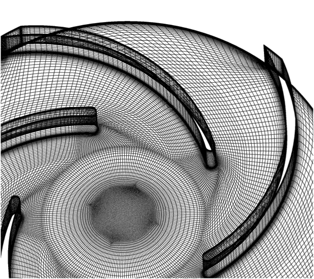
The centrifugal pump uses a spinning "impeller"
which has backward-swept blades.

The RANS model
The state of the art turbulence modelling is derived from averaging the Navier Stokes equation in time (Reynolds Averaged Navier Stokes, or RANS). During this averaging process the Reynolds stresses appear as additional unknown variables. Most models are based on the eddy viscosity concept, where the influence of turbulence fluctuations is modelled by the introduction of an additional eddy viscosity. These models are based on some crude assumptions and especially fail in strongly separated flows.

The LES model
Another approach for the computation of turbulent flow is the direct simulation of turbulence down to the grid size and modelling only turbulence at smaller scales. The LES (Large Eddy Simulation) approach requires very fine grids and time steps to resolve the important turbulent structures, which makes it unfeasible for high Reynolds number flows in complex industrial geometries.

The hybrid LES / RANS model
A mixed approach is hybrid LES / RANS modelling: a standard turbulence model is used for attached regions and switches to LES in strongly separated regions. This reduces the computational effort in comparison to pure LES and improves accuracy in comparison to pure RANS simulations.
Nevertheless, massive parallelization is required to solve the 3D transient simulation modell.


Data description
Each data set comprises one full rotation of the centrifugal pump consisting of 80 time steps. The numerical setup comprises 6.7 mio nodes and 6.4 mio cells, respectively. The setup contains 2 stationary domains (inlet and diffuser) and the moving rotor domain.

Because the hybrid models are the state-of-the-art today, two of the models we have chosen are from this class, namely DES and SAS.
DES was derived from the LES approach, while SAS is based on the URANS (= Unsteady RANS) approach.

The third model we have chosen, SST, is a model of the RANS class, which are the classical turbulence models, some of which exist for tens of years. We have chosen SST because it is one of the best in its class.

LES is (at least, currently) not feasible for complex geometries and high Reynolds numbers, because of the sheer amount of nodes necessary.

See our reference section for further information.

The visualization should look quite different when applied to the SST data set versus the other two hybrid models (DES and SAS): in the DES/SAS data sets, turbulent structures are resolved in massively separated regions. For this reason one should see much more detailed structures in comparison to the SST data set.

SST does not resolve turbulent fluctuations; only time-dependent average values can be computed. For the other two models turbulences can be directly resolved using a sufficiently dense grid.
 

Explaining the variables:
For each node, a couple of variables are available:

- pressure
- total pressure
- total pressure in stn frame
- turbulence kinetic energy
- velocity
- velocity in stn frame

Pressure: static pressure

Total pressure:
static pressure plus kinetic energy of the relative velocity in pressure units

Total pressure in stn frame (=Total pressure in 4):
static pressure plus kinetic energy of the absolute velocity

Turbulence kinetic energy (=Turbulence kinetic 5):
kinetic energy of the turbulent fluctuations of the velocity. Using SST, the whole turbulence is modeled (k-Omega model, k is the turbulent kinetic energy). With SAS or DES the modeled kinetic energy is clearly smaller as the turbulent fluctuations in the flow field are resolved.

Velocity:
velocity in the relative system (rotating with the impeller)

Velocity in stn frame (=Velocity in Stn Fr 7):
velocity in absolute system (observed from fixed generator casing).

Both velocities (velocity / velocity in stn frame) are differentiated only in the rotating part. In the stationary part, only one velocity exists. For example, if one would like to view the vortices within the impeller, the relative velocity has to be used. For questions regarding the energy transfer in balance equations, the absolute velocity is important.
As there are two different velocities, there are also two different formulations of the total pressure.

A word about the terms "absolute velocity" (= "velocity in stn frame") and "relative velocity" (new 15.06.2011)
First of all, all vectors and points are defined in a global Cartesian coordinate system, which is the same for all different kinds of velocity.
The fluid at a point p in space has some absolute velocity c.
If this point p is a point on the surface of the rotor, it moves on a circle around the axis of the rotor; this point p, then, has some other velocity u (which is exactly tangential to the circle). Thus, we can define the 'relative velocity' w of the fluid at p, which is w = c - u.

In other words, an observer sitting at p and moving along with p (but always looking in the same direction in the global coordinate system!) would observe the fluid in point p moving with a velocity w, while an observer sitting still relative to the global coordinate system would observe that same fluid in point p having velocity c.

The velocity of point p can be derived from the rotational velocity omega of the rotor by u = omega x r, where r is the vector from the rotor's axis to p (and perpendicular to the axis).

These notions can, of course, be extended to any point in the domain of the rotor. In addition, it is understood that all vectors and positions are functions of time.

PS: why would one want to express the same velocity in two different ways?
Because some differential equations are easier when expressed over the relative velocity, while others are easier when expressed over absolute velocity.

A word about the grids:
Even though the rotor physically moves in time with constant rotational speed, the flow inside the rotor is calculated with a stationary grid. The relative movement of rotor and stator domains is captured with the usage of transient rotor stator interfaces. The interface properly connects the nodes on both sides at rotated position.
For that reason the geometry is static for all files. (If the original data is post processed with CFX, the rotation of the grid is automatically done.) For any other tool the rotation needs to be done by the user. Despite the fact that rotation of the impeller is physical, analysis may be more appropriate for a stationary rotor depending on the task. Tracking the movement of vortical structures is easier without superposition of the rotation of the rotor.
For your information: the rotor domain contains all volume elements named with "ROTOR_VOL". It rotates with a velocity of -600 revolutions per minute around the Z axis (using the right-hand rule). The time step between two transient files is 1.25E-3 seconds, which corresponds to 4.5 degrees.

A bit more about the names of the elements:
The following surface elements are also part of the rotor volume:
- "Bodenscheibe",
- "Deckscheibe",
- "Deckscheibe Spalt",
- "LR Diffusor",
- "Schaufel",
- "Spalt Gehaeuse"

The following surface elements are the interfaces:
- "Eintritt Rotor 1 Side 2"
- "Eintritt Rotor 2 Side 2"
- "Rotor Diffusor Side 1"
- "Spalt SS Side 1"

File Formats
The data can be downloaded in two different formats,
Ansys 12.0 CFX and EnSight.

The Ansys CFX files might be useful for people already
having an Ansys license.

The EnSight files can be imported by many applications and libraries (e.g., VTK, ParaView, VisIt) and might also be useful for people who have already a EnSight license, or participants can use EnSight CFD Free edition, www.ensightcfd.com. EnSight standard trial licenses will be provided upon request (write an email to Eric O'Connell). EnSight CFD Free version does not require a license and can be simply downloaded and used without a license key.

The EnSight files are ASCII files, so they can be loaded
by home-grown visualization software. The files are in the EnSight Case Gold format, which is described in Chapter 12 of the EnSight User Manual, which can be downloaded here:

http://www.ensight.com/Download-document/180-User-Manual.html

If you would like to get a copy of the data in another format, please contact us, and we will see whether we can do something for you.

Test data
If you would like to develop your own loader for the
EnSight files, you might want to test your loader with
the following toy example.

EnSight Gold file format: download

Visualization of the test data. In this case, the scalar "Eddy_Viscosity" is used.

Contest data

All 3 data sets in both formats (CFX / EnSight) can be downloaded from following two locations

• SDSC Cloud
• Kitware Server